Primitives
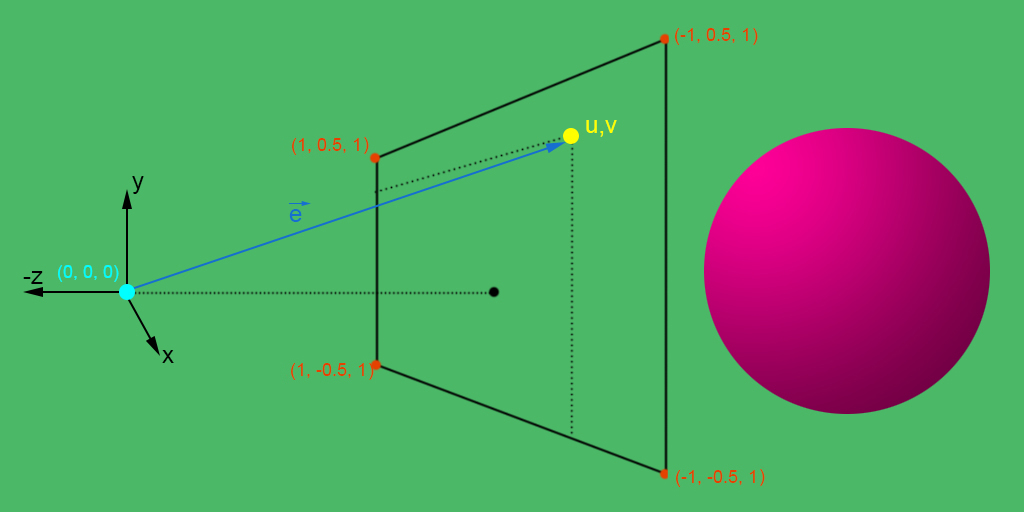
The first thing is to define the ray origin $O$ and direction $\large ê$, where the unit vector $\large ê = \frac{\vec{e}}{\parallel \vec{e} \parallel}$.

Implementation of ray-sphere intersection algorithm.
%matplotlib inline
import matplotlib
import matplotlib.pyplot as plt
import numpy as np
np.seterr(divide='ignore', invalid='ignore')
plt.rcParams['figure.figsize'] = (16, 4)
The first thing is to define the ray origin $O$ and direction $\large ê$, where the unit vector $\large ê = \frac{\vec{e}}{\parallel \vec{e} \parallel}$.

## Ray
O = np.array([0, 0])         # Origin pont
e_ = np.array([0.5, 0.5])    # Ray direction
e_ /= np.linalg.norm(e_)     # Unit vector of e_
Next step is to define the sphere/circle center $C_s$ and radius $\large r$.

# Sphere
Cs = np.array([2, 0])        # Center of sphere
r = 1.5                      # Radius of sphere
To find the ray intersection, the next step is define the oriented segment $\overline{OC} = Cs - O$. 
OC_ = Cs - O # Oriented segment from origin to center of the sphere
Next step, we need to find the parameter $\large t$ which will parametrize the ray segment and find the intersections from the origin. The value $\large t$ can be found by projecting the vetor $\vec{OC}$ on the versor $\large ê$. The projection of a vector $\large \vec{a}$ on a $\large \vec{b}$ can be defined as the geometric representation of dot product:
$$ \large a_1 = \parallel a \parallel \cos{\theta} = a \cdot \hat{b} = a \cdot \frac{\vec{b}}{\parallel \vec{b} \parallel} $$
t = np.dot(OC_, e_) # Vector projection of OC_ on e_
Having the parameter $\large t$, we can finally define the segment which will give us the point $P_e$ projected from center of the sphere on the ray direction. Applying the concept of parametrized line, we can define:
$$ \large P_e = O + t \cdot \hat{e} $$Having this point, we can find the distance between $C_s$ and $P_e$ with ${\parallel P_e - C_s \parallel}_2$.

Pe = O + e_*t                # Point on vector e_ projected from OC_
d = np.linalg.norm(Pe - Cs)  # Distance from the point Pe and the center of the sphere
Notice that now we have the distance $\large d$ so we can make some assumptions:

Now we have all the necessary to calculate the intersection positions using the pythagorean theorem se we can have the value $\large i$ and define the positions based on the parametrized line from origin.
$$ \large \begin{aligned} P_s^1 & = O + \hat{e} \cdot (t - i) \\ P_s^2 & = O + \hat{e} \cdot (t + i) \end{aligned} $$
# Position of the intersections
if(d > r):
    print("No intersection!")

elif(d == r):
    Ps = Pe
    print(f'Intersection at {Ps}')

else:
    i = (r**2 - d**2)**0.5
    Ps1 = O + e_*(t - i)
    Ps2 = O + e_*(t + i)
    print(f'Intersections at {Ps1} and {Ps2}')
Intersections at [0.64644661 0.64644661] and [1.35355339 1.35355339]
fig, ax = plt.subplots(figsize=(16, 10))

# Define x points to draw lines
x = np.array([0, 8])
colors = ["red", "green", "blue", "brown","orange"]

# Define angular coeficients
M = [0, 0.25, 0.5, 1, 1.5]

# Define sphere
Cs = [4, 2]
r = 2
Circle = plt.Circle(Cs, r, color="k", fill=0)
ax.add_artist(Circle)

# Draw intersections
for index, m in enumerate(M):
    y = m*x
    plt.plot(x, y, color=colors[index])
    plt.xlim([-0.1, 8])
    plt.ylim([-0.1, 5])

    # Define ray
    O = np.array([0, 0])
    e_ = np.array([1, m])
    e_ = e_/np.linalg.norm(e_)

    # Intersection
    OC_ = Cs - O
    t = np.dot(OC_, e_)
    Pe = O + e_*t
    d = np.linalg.norm(Pe - Cs)

    # Draw intersections
    if(d == r):
        Ps = Pe
        Circle = plt.Circle(Ps, 0.1, color=colors[index], fill=0)
        ax.add_artist(Circle)
    if(d < r):
        i = (r**2 - d**2)**0.5
        Ps1 = O + e_*(t - i)
        Circle = plt.Circle(Ps1, 0.1, color=colors[index], fill=0)
        ax.add_artist(Circle)
        Ps2 = O + e_*(t + i)
        Circle = plt.Circle(Ps2, 0.1, color=colors[index], fill=0)
        ax.add_artist(Circle)

plt.show()
Apply same model for each pixel of an image plane as the origin and the ray direction is based on the perspective camera model:

N, M = 256j, 512j
O = np.ones((int(N.imag), int(M.imag), 3))               # Init image plane origin
O[..., 1], O[..., 0] = np.mgrid[0.5:-0.5:N, 1:-1:M]      # Image plane uvw coordinates
e_ = O/np.linalg.norm(O, axis=2)[:,:,np.newaxis]         # Normalized ray directon e_

# Sphere
Cs = np.array([0, 0, 4])                                 # Center of sphere
r = 1.5                                                  # Radius of sphere

OC_ = Cs - O                                             # Oriented segment from origin to center of the sphere

vec_dot = np.vectorize(np.dot, signature='(n),(m)->()')  # Vectorize dot product function
t = vec_dot(OC_, e_)                                     # Pixelwise dot product
Pe = O + e_*t[:,:,np.newaxis]                            # Point on vector e_ projected from OC_
d = np.linalg.norm(Pe - Cs, axis=2)                      # Distance from the point Pe and the center of the sphere

# Find intersection position
i = (r**2 - d**2)**0.5                                   #
Ps = O + e_*(t - i)[:,:,np.newaxis]                      #

# Facing ratio (incidence value)
i_ = i[:,:,np.newaxis]/r

# Calculate the normal vector for each point
n = Ps - Cs                                              # Calculate vector n
n_ = n/np.linalg.norm(n, axis=2)[:,:,np.newaxis]         # Normalize n


##################################
# Simple directional light model #
##################################
Cd = np.array([0.9, 0.15, 0.35])**(1/0.455)              # Sphere diffuse color with gamma compensation

# Key light
l = np.array([-1.5, 1.5, -1])                            # Key light vector
l_ = l/np.linalg.norm(l)                                 # Key light vector normalization
Kd = vec_dot(l_, n_)[:,:,np.newaxis]                     # Calculate light incidence
Kd[Kd < 0] = 0                                           # clamp negative values
diff = Cd*Kd                                             # Writes to diffuse

# Back light
l = np.array([1.5, -1, 1])                               # Back light vector
l_ = l/np.linalg.norm(l)                                 # Back light vector normalization
Kd = vec_dot(l_, n_)[:,:,np.newaxis]                     # Calculate light incidence
Kd[Kd < 0] = 0                                           # clamp negative values
diff += Cd*Kd*0.25                                       # Adds to diffuse

output = np.zeros((int(N.imag), int(M.imag), 3))         # Init output image
output[d < r] = (diff*i_)[d < r]                         # Shades diffuse and fr

output[output < 0] = 0; output[output > 1] = 1           # Clamp values before visualization


# Visualization
fig, ax = plt.subplots(figsize=(16, 10))
ax.imshow(output**(1/2.2))                               # View the resulting image with gamma adjustment (sRGB)
plt.show()