Examples of animated visualization using Matplotlib.
%matplotlib inline
import matplotlib.pyplot as plt
from matplotlib import cm
import numpy as np
from numba import jit
import imageio as iio
import os, sys
import matplotlib.animation as manim
plt.rcParams['figure.figsize'] = (16, 8)
Matplotlib is probably the most popular data/scientific visualization library for python. Despite normally working with static figures, it also provides some decent ways to produce moving imaging. Let’s take a look in how to export visually our animated data.
To export an image sequence you basically have to loop through a batch of functions which are responsible for saving our Matplotlib’s imshows. After getting the picture sequence (ordered or not), we are able to produce videos, GIFs or any kind of moving visual image media by using editors such as Gimp, Photoshop, After Effects and so one.
For this example, we have a sequence of pictures like image.0000.png
, image.0001.png
… image.0008.png
, similar to the following example, which shows us the color hue shifting of a given input image.
fig, (axA, axB) = plt.subplots(1, 2)
imgA = iio.imread('../_data/babuino.png')/255
frames = 4
for frame in range(frames):
imgA = (imgA + frame/frames) % 1
axA.imshow(imgA)
axB.hist(imgA[..., 0].ravel(), bins=256, range=(0.0, 1.0), fc='r', alpha=0.5)
axB.hist(imgA[..., 1].ravel(), bins=256, range=(0.0, 1.0), fc='g', alpha=0.5)
axB.hist(imgA[..., 2].ravel(), bins=256, range=(0.0, 1.0), fc='b', alpha=0.5)
plt.tight_layout()
plt.savefig('output/matplotlib_animation_colorShift.{0:04d}.png'.format(frame))
axA.cla(); axB.cla()
plt.close()
%%HTML
<table>
<tr>
<td><img src='output/matplotlib_animation_colorShift.0000.png' width="512"></td>
<td><img src='output/matplotlib_animation_colorShift.0001.png' width="512"></td>
</tr>
<tr>
<td><img src='output/matplotlib_animation_colorShift.0002.png' width="512"></td>
<td><img src='output/matplotlib_animation_colorShift.0003.png' width="512"></td>
</tr>
</table>
![]() | ![]() |
![]() | ![]() |
Before exporting GIFs, we have to install a free and open source software called ImageMagick, which is going to work together with Matplotlib’s animation module. To install ImageMagick on Linux and OSX, run the following command:
$ sudo apt install imagemagick
or
$ conda install --channel conda-forge imagemagick
For windows folow ImageMagick download.
# windows user only
plt.rcParams["animation.convert_path"] = "C:\ProgramFiles\ImageMagick\magick.exe"
@jit(nopython=True, parallel=True)
def nabla2f(Z):
'''
Laplace operator
'''
Zup = Z[0:-2,1:-1]
Zdown = Z[2:,1:-1]
Zleft = Z[1:-1,0:-2]
Zright = Z[1:-1,2:]
Zcenter = Z[1:-1,1:-1]
return Zup + Zleft + Zdown + Zright - 4*Zcenter
@jit(nopython=True, parallel=True)
def reactionDiffusion(U, V, u, v, ru, rv, f, k, iters):
'''
Reaction diffusion system
'''
for i in range(iters):
u += ru*nabla2f(U) - u*v**2 + f*(1 - u)
v += rv*nabla2f(V) + u*v**2 - (f + k)*v
return V
fig, ax = plt.subplots(figsize=(2048//72, 512//72))
# gif parameters
N1, N2 = 128j, 512j
M1, M2 = int(N1.imag), int(N2.imag)
iters = 70
frames = 30
# RD system initialization
np.random.seed(sum(map(lambda c: ord(c), 'reaction diffusion')))
U = np.zeros((M1 + 2, M2 + 2)); u = U[1:-1, 1:-1]
V = np.zeros((M1 + 2, M2 + 2)); v = V[1:-1, 1:-1]
t, s = np.mgrid[-0.25:0.25:N1, -1:1:N2]
fo = 5
u += np.sin(np.pi*s*fo)*np.sin(np.pi*t*fo) >= 2**0.5/2
v += np.cos(np.pi*s*fo)*np.cos(np.pi*t*fo) >= 2**0.5/2
e = 0.4
u += np.random.random((M1, M2))*e - e
v += np.random.random((M1, M2))*e - e
f, k, ru, rv = 0.06, 0.062, 0.19, 0.05
def animation(frame):
plt.cla(); #ax.set_ylim(-1, 1); ax.set_title('White Noise')
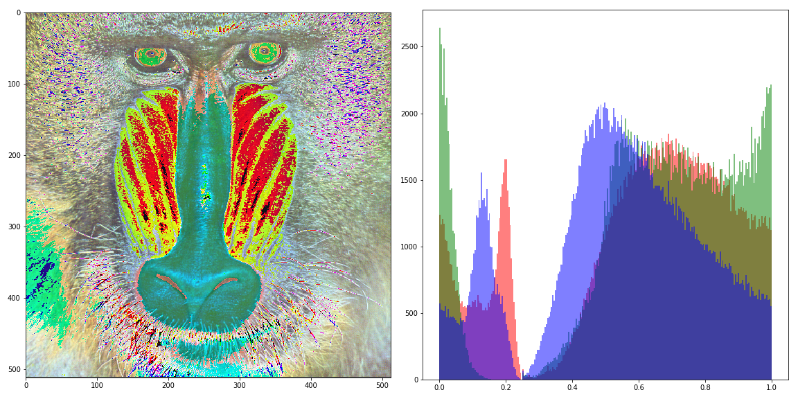
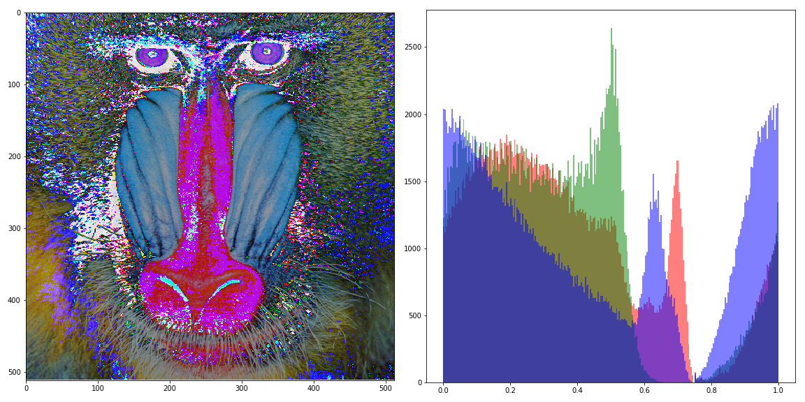
RD = reactionDiffusion(U, V, u, v, ru, rv, f, k, iters)
imshow = ax.imshow(RD, vmin=RD.min(), vmax=RD.max())
plt.tight_layout()
return imshow
anim = manim.FuncAnimation(fig, animation, frames=30, interval=100)
anim.save('output/matplotlib_animation_reactionDiffusion.gif', writer="imagemagick", extra_args="convert")
plt.close()
# Solve repetition problem
! magick convert _output/matplotlib_animation_reactionDiffusion.gif -loop 0 _output/matplotlib_animation_reactionDiffusion.gif
! echo GIF exported and reconverted. Disregard the message above.
MovieWriter imagemagick unavailable.
GIF exported and reconverted. Disregard the message above.
On the same way of GIFs exportation, we have to install an extra dependency to work together with Matplotlib’s animation module. In this instance, the well-known FFmpeg is maybe our best choice (at least as far as I know). To install this on Linux and OSX, run:
$ sudo apt-get install ffmpeg
or
$ conda install --channel conda-forge ffmpeg
For this example, we are going to produce an animated 2D Bandpass Filter. First step is to load an image and get its spectrum.
img = iio.imread('../_data/barco.png')/255
IMG = np.fft.fft2(img)
IMG = np.fft.fftshift(IMG)
fig, (axA, axB) = plt.subplots(1, 2)
axA.imshow(img, cmap='gray')
axA.set_title('input image')
axB.imshow(np.log10(1 + abs(IMG)), cmap='gray')
axB.set_title('spectrum')
plt.show()
t, s = np.mgrid[-1:1:512j, -1:1:512j]
d = (s**2 + t**2)**0.5
f = lambda mu, sigma: 1/(sigma*(2*np.pi)**0.5)*np.exp(-1/2*((d - mu)/sigma)**2)
FFMpegWriter = manim.writers['ffmpeg']
metadata = dict(title='Band-pass filter', artist='Diego Inácio',
comment='Exporting movies using Python and Matplotlib')
writer = FFMpegWriter(fps=15, metadata=metadata)
fig, (axA, axB) = plt.subplots(1, 2)
mu, sigma = -0.5, 0.1
frames = 90
with writer.saving(fig, 'output/matplotlib_animation_BPF.mp4', frames):
for i in range(frames):
H = f(mu, sigma)
axA.imshow(H, cmap='gray')
axA.set_title(r'filter H, $\sigma={0}$, $\mu={1:.2f}$'.format(sigma, mu))
img_H = np.fft.ifftshift(H*IMG)
img_H = np.fft.ifft2(img_H).real
axB.imshow(img_H, cmap='gray')
axB.set_title('filtered image')
mu += 2/frames
writer.grab_frame()
print('{:06.2f} %'.format(100*(i + 1)/frames), end='\r', flush=True)
plt.close()
100.00 %
%%HTML
<video width='900' height='450' controls>
<source src='output/matplotlib_animation_BPF.mp4' type='video/mp4'>
</video>