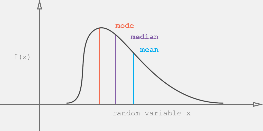
Overview of location measures and central tendency of data.
Measures of location are a means of acquiring and describing the central tendency of a certain amount of data or distribution. The most common are mean, median and mode, despite these may be called as "average" (more formally, a measure of central tendency).
%matplotlib inline
import matplotlib
import matplotlib.pyplot as plt
import numpy as np
The arithmetic mean (or simply mean or average) can be described as the sum of all measurements divided by the number of observations in the data set.
$$ \large \displaystyle \frac{1}{n} \sum_{i=1}^{n} x_i = \frac{x_1+x_2+\cdots+x_n}{n} $$For example, given the list of 5 numbers: $5, 87, 45, 32, 1$
The arithmetic mean of this observation would be:
$$ \large \displaystyle \frac{5 + 87 + 45 + 32 + 1}{5} = \frac{170}{5} = 34 $$numbers = np.array([5, 87, 45, 32, 1])
arithmetic_mean = numbers.sum()/numbers.size
print(arithmetic_mean)
34.0
The geometric mean can be described the nth root of the product of all observations in the data set.
$$ \large \displaystyle \left(\prod_{i=1}^{n} x_i\right)^{\frac{1}{n}} = \sqrt[n]{x_1 \cdot x_2 \cdots x_n} $$This location measure is valid only for data that are measured absolutely on a strictly positive scale (values grather than zero).
$$ \large \displaystyle \mathbb{Z}_{>0} := \{x \in \mathbb{Z}:x > 0\} $$For example, given the same list of 5 numbers: $5, 87, 45, 32, 1$
The geometric mean of this observation would be:
$$ \large \displaystyle \sqrt[\leftroot{-2}\uproot{2}5]{5 \cdot 87 \cdot 45 \cdot 32 \cdot 1} = \sqrt[\leftroot{-2}\uproot{2}5]{626400} \approx 14.4 $$numbers = np.array([5, 87, 45, 32, 1])
geometric_mean = numbers.prod()**(1/numbers.size)
print(geometric_mean)
14.433456571308836
The harmonic mean can be described as the reciprocal arithmetic mean of the reciprocals of the data values. In the same way as the geometric mean, this location measure is valid only for data that are measured absolutely on a strictly positive scale (values grather than zero).
$$ \large \displaystyle \frac{n}{\sum_{i=1}^{n} \frac{1}{x_i}} = \frac{n}{\frac{1}{x_1}+\frac{1}{x_2}+\cdots+\frac{1}{x_n}} $$For example, given the same list of 5 numbers: $5, 87, 45, 32, 1$
The harmonic mean of this observation would be:
$$ \large \displaystyle \frac{5}{\frac{1}{5}+\frac{1}{87}+\frac{1}{45}+\frac{1}{32}+\frac{1}{1}} = \frac{5}{\frac{8352+480+928+1305+41760}{41760}} = \frac{5}{\frac{52825}{41760}} = \frac{208800}{52825} \approx 3.95 $$numbers = np.array([5, 87, 45, 32, 1])
harmonic_mean = 5/np.sum(1/numbers)
print(harmonic_mean)
3.952673923331756
The power mean is a kind of generalized mean that is basically an abstraction of the quadratic, arithmetic, geometric and harmonic means.
$$ \large \displaystyle \left(\frac{1}{n} \sum_{i=1}^{n} x_i^p\right)^{\frac{1}{p}} = \sqrt[p]{\frac{{x_1^p+x_2^p+\cdots+x_n^p}}{n}} $$The expoent $\large p$ is the parameter that allows us to change its behavior. By choosing different values for the parameter $\large p$, the following types of means are obtained:
$$ \large \displaystyle \begin{align} p &\rightarrow - \infty & \text{minimum value} \\ p &= -1 & \text{harmonic mean} \\ p &\rightarrow 0 & \text{geometric mean} \\ p &= +1 & \text{arithmetic mean} \\ p &\rightarrow + \infty & \text{maximum value} \\ \end{align} $$numbers = np.array([5, 87, 45, 32, 1])
f = lambda p: (np.sum(numbers**p)/numbers.size)**(1/p)
# minimum value (p tends to minus infinity)
p = -150.0
print("minimum value: ", f(p))
# harmonic mean
p = -1.0
print("harmonic mean: ", f(p))
# geometric mean (p approximates to zero)
p = 0.00000000001
print("geometric mean: ", f(p))
# arithmetic mean
p = 2.0
print("arithmetic mean: ", f(p))
# maximum value (p tends to infinity)
p = 150.0
print("maximum value: ", f(p))
minimum value: 1.010787354517243 harmonic mean: 3.9526739233317563 geometric mean: 14.43352271139387 arithmetic mean: 46.138920663578595 maximum value: 86.07151604261179
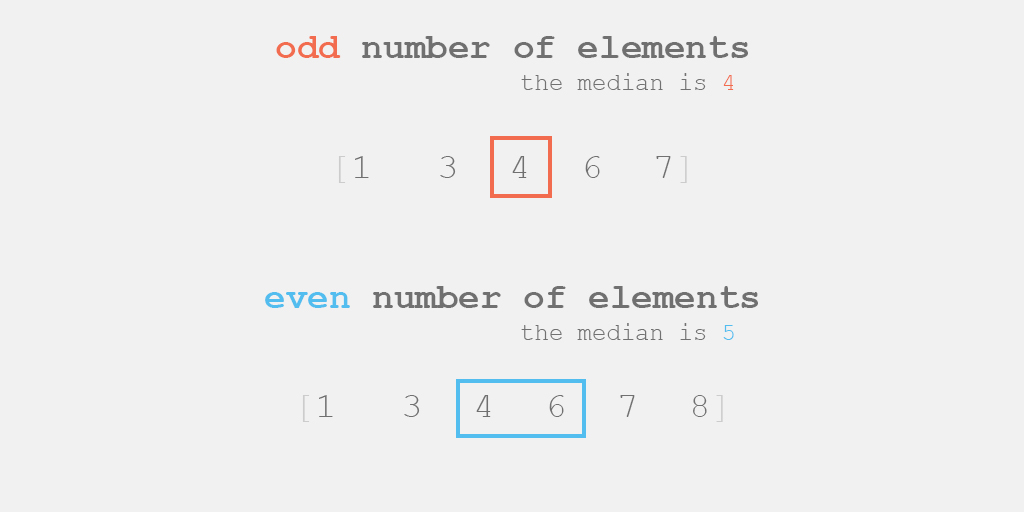
The median measure is basically the way to find the middle point of a data set, which means it divides the observations into two halves. The mothod to reach these values follows two basic steps. Firstly, arrange the values in an ascending order (or descending.. it does not make any difference in this case). And finally, gets the middle value of the data. If data has odd number of elements, it is the middle element (or $\frac{n}{2}$th element). If data has even number of elements, it is the mean of the two center data ($\frac{n}{2}$th and $\left[\frac{n}{2} + 1\right]$th).
For example, given the list of 5 numbers: $5, 87, 45, 32, 1$
The first step is to sort all the elements: $1, 5, 32, 45, 87$
Finally, get the middle element, which in this case (odd number of elements) is the value $32$.
numbers = np.array([5, 87, 45, 32, 1])
numbers_sort = np.sort(numbers)
# the 3rd element has index 2
middle = numbers_sort.size//2
median = numbers_sort[middle]
print(median)
32
For another example, lets take a list of 6 numbers: $5, 87, 45, 32, 1, 38$
The first step is to sort all the elements: $1, 5, 32, 38, 45, 87$
Finally, get the center elements, which in this case (even number of elements) are $32$ ($\frac{n}{2}$) and $38$ ($\frac{n}{2} + 1$). Thus, the median value is $35$ ($\frac{32 + 38}{2}$).
numbers = np.array([5, 87, 45, 32, 1, 38])
numbers_sort = np.sort(numbers)
# the 3rd and 4th elements have indices 2 and 3, respectively
middle = numbers_sort.size//2
median = (numbers_sort[middle - 1] + numbers_sort[middle])/2
print(median)
35.0
The mode measure is the method to find the most frequent value in a data set. Any set of data can have one or more modes, which it is named as bimodal (2 modes) or multimodal (more than 2 modes). The mode measure is the only central tendency measure that can be used with nominal data, which have purely qualitative category assignments.
For example, given a list of elements: $4, 6, 4, 6, 8, 7, 9, 10, 6$
To make to process more visually intuitive, lets firstly sort this list: $4, 4, 6, 6, 6, 7, 8, 9, 10$
And after, lets build a frequency table:
value | number of occurrences |
---|---|
4 | 2 |
6 | 3 |
7 | 1 |
8 | 1 |
9 | 1 |
10 | 1 |
Given that, the mode value is $6$, which has the highest number of occurrences (3).
elements = [4, 6, 4, 6, 8, 7, 9, 10, 6]
elements_sort = sorted(elements)
occurrences = {e: elements.count(e) for e in set(elements)}
highest_occ = max(occurrences.values())
mode = [e for [e, n] in occurrences.items() if n >= highest_occ]
print("elements: ", elements)
print("sorted: ", elements_sort)
print("occurrences: ", occurrences)
print("mode: ", mode)
elements: [4, 6, 4, 6, 8, 7, 9, 10, 6] sorted: [4, 4, 6, 6, 6, 7, 8, 9, 10] occurrences: {4: 2, 6: 3, 7: 1, 8: 1, 9: 1, 10: 1} mode: [6]
For another example, lets take a list of nominal elements: Brazil, Argentina, Brazil, Argentina, Chile, Argentina, Chile, Peru, Brazil, Argentina, Brazil
And after, lets build a frequency table:
value | number of occurrences |
---|---|
Brazil | 4 |
Argentina | 4 |
Chile | 2 |
Peru | 1 |
Given that, the mode are Argentina and Brazil, since they have the same number of occurrences (4). In other words, this measure is bimodal.
elements = ["Brazil", "Argentina", "Brazil", "Argentina", "Chile", "Argentina", "Chile", "Peru", "Brazil", "Argentina", "Brazil"]
occurrences = {e: elements.count(e) for e in set(elements)}
highest_occ = max(occurrences.values())
mode = [e for [e, n] in occurrences.items() if n >= highest_occ]
print("elements: ", elements)
print("occurrences: ", occurrences)
print("mode: ", mode)
elements: ['Brazil', 'Argentina', 'Brazil', 'Argentina', 'Chile', 'Argentina', 'Chile', 'Peru', 'Brazil', 'Argentina', 'Brazil'] occurrences: {'Brazil': 4, 'Argentina': 4, 'Peru': 1, 'Chile': 2} mode: ['Brazil', 'Argentina']