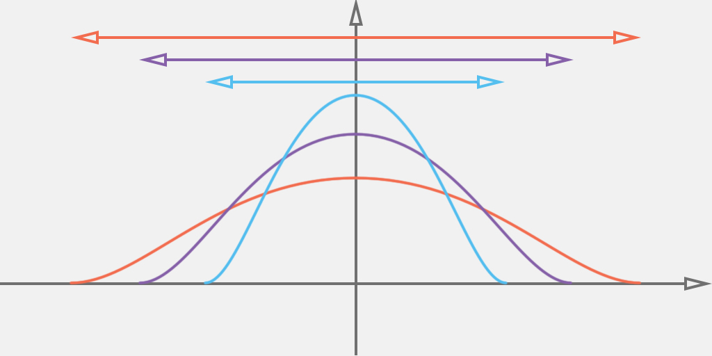
Measures of dispersion are a means of describing the spread of a certain amount of data or distribution. They include range, variance, deviation, coeficient of variation and so on.

Overview of dispersion measures in statistics.
Measures of dispersion are a means of describing the spread of a certain amount of data or distribution. They include range, variance, deviation, coeficient of variation and so on.

%matplotlib inline
import matplotlib
import matplotlib.pyplot as plt
import numpy as np
The range measure is basically the absolute difference between the lowest and the highest values in a data set. Therefore, to obtain this result, only the minimum and the maximum values are needed.
For example, given a list of elements: $17,10,9,21,14,13,18,12,8,20,15$
To make to process more visually intuitive, lets firstly sort this list: $8,9,10,12,13,14,15,17,18,20,21$
The next step is to find the minimum and the maximum values, which are $8$ and $21$, respectivelly.
Finally, subtract the minimum from the maximum.
$$ \large max - min = 21 - 8 = 13 $$elements = np.array([17, 10, 9, 21, 14, 13, 18, 12, 8, 20, 15])
elements_sort = np.sort(elements)
minimum = elements_sort.min()
maximum = elements_sort.max()
range = maximum - minimum
print("elements: ", elements)
print("sorted: ", elements_sort)
print("minimum: ", minimum)
print("maximum: ", maximum)
print("range: ", range)
elements:  [17 10  9 21 14 13 18 12  8 20 15]
sorted:  [ 8  9 10 12 13 14 15 17 18 20 21]
minimum:  8
maximum:  21
range:  13
Another very well know range measure is the interquartile range, which basically substitute the minimum and the maximum values with the $Q_1$ and $Q_3$, respectively. Using the same value list from the latest example, we have:
$$ \large Q_3 - Q_1 = 18 - 10 = 8 $$elements = np.array([17, 10, 9, 21, 14, 13, 18, 12, 8, 20, 15])
elements_sort = np.sort(elements)
n = elements.size
Q1 = np.median(elements_sort[:n//2])
Q3 = np.median(elements_sort[n//2 + 1:])
interquartile_range = Q3 - Q1
print("elements: ", elements)
print("sorted: ", elements_sort)
print("Q1: ", Q1)
print("Q3: ", Q3)
print("interquartile_range: ", interquartile_range)
elements:  [17 10  9 21 14 13 18 12  8 20 15]
sorted:  [ 8  9 10 12 13 14 15 17 18 20 21]
Q1:  10.0
Q3:  18.0
interquartile_range:  8.0
The mean absolute deviation, variance and the standard deviation are a kind of measure based on the dissimilarity of each element value in relation to the arithmetic mean value ($\large \mu$ or $\large \overline{x}$) of the data set. A very important point here is to distinguish the sample measure from the population measure:
| Sample | Population | |
|---|---|---|
| Mean Absolute Deviation | $$\large MAD=\frac{\sum \mid x_i - \overline{x} \mid}{n}$$ | $$\large MAD=\frac{\sum \mid x_i - \mu \mid}{n}$$ |
| Variance | $$\large s^2=\frac{\sum (x_i - \overline{x})^2}{n-1}$$ | $$\large \sigma^2=\frac{\sum (x_i - \mu)^2}{n}$$ |
| Standard Deviation | $$\large s=\sqrt{\frac{\sum (x_i - \overline{x})^2}{n-1}}$$ | $$\large \sigma=\sqrt{\frac{\sum (x_i - \mu)^2}{n}}$$ |
where:
For example, given a list of ages of randomly selected voters: $19, 21, 34, 20, 55, 43, 22, 36$
Firstly, lets calculate the arithmetic mean:
$$ \large \overline{x} = \frac{\sum x_i}{n} = \frac{19+21+34+20+55+43+22+36}{8} = \frac{240}{8} = 30 $$Now we are able to calculate the Mean Absolute Deviation:
$$ \begin{align} MAD&=\frac{\sum \mid x_i - \overline{x}\mid }{n} \\ MAD&=\frac{\mid 19 - 30 \mid + \mid 21 - 30 \mid + \mid 34 - 30 \mid + \mid 20 - 30 \mid + \mid 55 - 30 \mid + \mid 43 - 30 \mid + \mid 22 - 30 \mid + \mid 36 - 30 \mid }{8} \\ MAD&=\frac{84}{8} \\ MAD& = 10.5 \end{align} $$Considering our data as a sample, the variance value would be:
$$ \begin{align} s^2&=\frac{\sum (x_i - \overline{x})^2}{n-1} \\ s^2&=\frac{(19 - 30)^2 + (21 - 30)^2 + (34 - 30)^2 + (20 - 30)^2 + (55 - 30)^2 + (43 - 30)^2 + (22 - 30)^2 + (36 - 30)^2}{8 - 1} \\ s^2&=\frac{1192}{7} \\ s^2& \approx 170.29 \end{align} $$Having that, the standard deviation is calculated as the square root of the variance.
$$ \large s = \sqrt{s^2} = \sqrt{170.29} \approx 13.05 $$elements = np.array([19, 21, 34, 20, 55, 43, 22, 26])
n = elements.size
mean = np.sum(elements)/n
mad = np.sum(np.absolute(elements - mean))/n
variance = np.sum((elements - mean)**2)/(n - 1)
std = (np.sum((elements - mean)**2)/(n - 1))**0.5
print("elements: ", elements)
print("mean: ", mean)
print("mean absolute deviation: ", mad)
print("variance: ", variance)
print("standard deviation: ", std)
elements:  [19 21 34 20 55 43 22 26]
mean:  30.0
mean absolute deviation:  10.5
variance:  170.28571428571428
standard deviation:  13.04935685333627
For another example, lets take the grades of all the 8 students of a class: $7.5, 8, 7, 9.5, 9, 8.5, 7.5, 7$
Now, lets calculate the arithmetic mean:
$$ \large \mu = \frac{\sum x_i}{n} = \frac{7.5+8+7+9.5+9+8.5+7.5+7}{8} = \frac{64}{8} = 8 $$The mean absolute deviation would be:
$$ \begin{align} MAD&=\frac{\sum \mid x_i - \mu \mid }{n} \\ MAD&=\frac{\mid 7.5 - 8 \mid + \mid 8 - 8 \mid + \mid 7 - 8 \mid + \mid 9.5 - 8 \mid + \mid 9 - 8 \mid + \mid 8.5 - 8 \mid + \mid 7.5 - 8 \mid + \mid 7 - 8 \mid }{8} \\ MAD&=\frac{6}{8} \\ MAD& = 0.75 \end{align} $$Considering our data represents the whole population, the variance value would be:
$$ \begin{align} \sigma^2&=\frac{\sum (x_i - \mu)^2}{n} \\ \sigma^2&=\frac{(7.5 - 8)^2 + (8 - 8)^2 + (7 - 8)^2 + (9.5 - 8)^2 + (9 - 8)^2 + (8.5 - 8)^2 + (7.5 - 8)^2 + (7 - 8)^2}{8} \\ \sigma^2&=\frac{6}{8} \\ \sigma^2& = 0.75 \end{align} $$Having that, the standard deviation is calculated as the square root of the variance.
$$ \large \sigma = \sqrt{\sigma^2} = \sqrt{0.75} \approx 0.87 $$elements = np.array([7.5, 8, 7, 9.5, 9, 8.5, 7.5, 7])
n = elements.size
mean = np.sum(elements)/n
mad = np.sum(np.absolute(elements - mean))/n
variance = np.sum((elements - mean)**2)/n
std = (np.sum((elements - mean)**2)/n)**0.5
print("elements: ", elements)
print("mean: ", mean)
print("mean absolute deviation: ", mad)
print("variance: ", variance)
print("standard deviation: ", std)
elements:  [7.5 8.  7.  9.5 9.  8.5 7.5 7. ]
mean:  8.0
mean absolute deviation:  0.75
variance:  0.75
standard deviation:  0.8660254037844386
The coeficient of variation (or relative standard deviation) is basically a measure of the extent of variability in relation to the absolute mean value ($\large |\mu|$). In other words, how far from the average the data points are. It can be simply defined as the ration between the standard deviation and the mean.
$$ \large c_v = \frac{\sigma}{\mu} $$Given the same grades of all the 8 students of a class from our latest example: 7.5,8,7,9.5,9,8.5,7.5,7
We already know that the standard deviation $\large \sigma$ and absolute mean $\large \mu$ are 0.87 and 8, respectively. In this way, we have:
$$ \large c_v = \frac{\sigma}{\mu} = \frac{0.87}{8} \approx 0.11 $$elements = np.array([7.5, 8, 7, 9.5, 9, 8.5, 7.5, 7])
n = elements.size
mean = np.sum(elements)/n
std = (np.sum((elements - mean)**2)/n)**0.5
cv = std/mean
print("elements: ", elements)
print("mean: ", mean)
print("standard deviation: ", std)
print("coeficient of variation: ", cv)
elements:  [7.5 8.  7.  9.5 9.  8.5 7.5 7. ]
mean:  8.0
standard deviation:  0.8660254037844386
coeficient of variation:  0.10825317547305482