Number of set elements
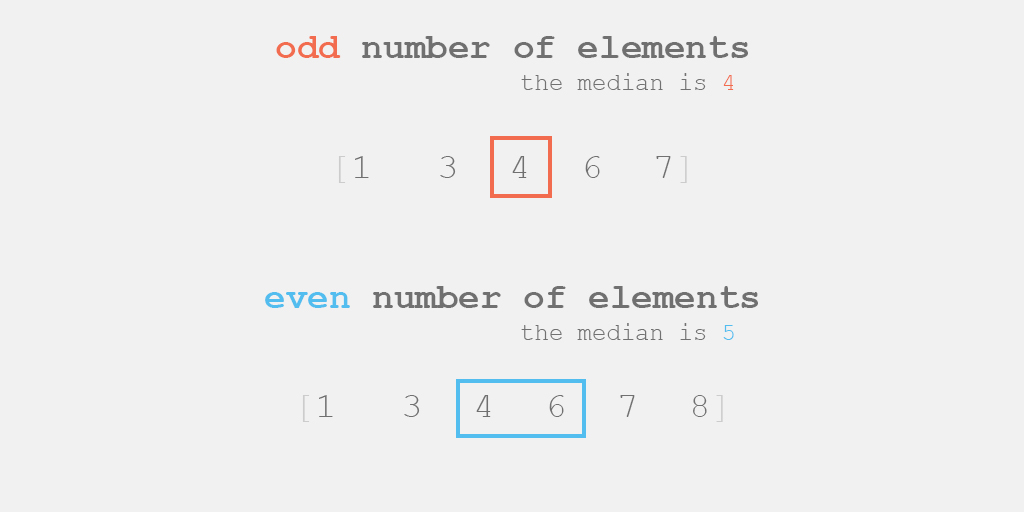
In the same way as in measures of central tendency, the number of set elements matters here. For example, if data has odd number of elements, it is the middle element (or $\frac{n}{2}$ th element). If data has even number of elements, it is the mean of the two center data ($\frac{n}{2}$ th and $\left[ \frac{n}{2} + 1 \right]$th).

However, sometimes (depending on the number of elements) the point of our measure of position is not exactly in the middle of 2 elements. Sometimes it falls closer to one than the other, so we have to interpolate those values in order to find the weighted result. Firstly, let's use a quantile value $q$, which ranges from 0 to 1.
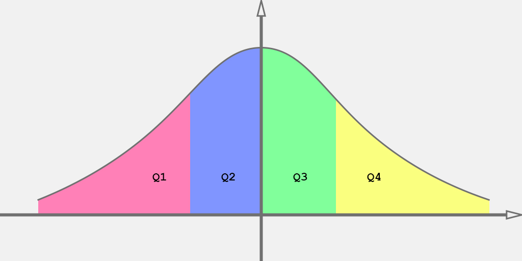
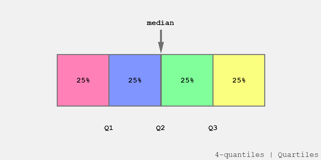
- $Q_1$ is the first quartile and $q = 0.25$;
- $Q_3$ is the third quartile and $q = 0.75$;
- $D_4$ is the fourth decile and $q = 0.4$;
- $P_8$ is the eighth percentile and $q = 0.08$;
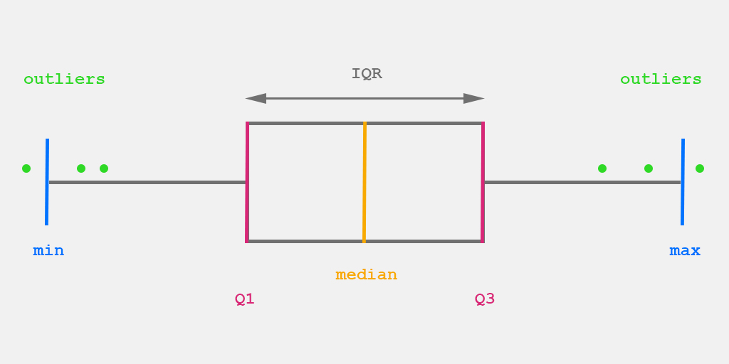
- $q = 0$ and $q = 1$ are the minimum and maximum values, respectively.
Having the quantile value, we can find the position value $p$ as:
$$ \large p = q \cdot (n - 1) $$
where $n$ is the number of elements in the set. Thus:
- If $p = 0.25$ the point is between the elements 0 and 1;
- If $p = 1.75$ the point is between the elements 1 and 2;
- If $p = 5.01$ the point is between the elements 5 and 6;
- If $p = 11.99$ the point is between the elements 11 and 12.
Considering our value $p$ falls between two elemens $a$ and $b$, the interpolated value $I$ can be:
$$ \large t = a - p \quad ; \quad I = (1 - t) \cdot v_a + t \cdot v_b $$
where $v_a$ and $v_b$ are the values of the elements $a$ and $b$, respectively.
For example, given the list of 6 numbers: 5, 87, 45, 32, 1, 38
The next step is to sort all the elements: 1, 5, 32, 38, 45, 87
If we want to calculate the first quartile ($Q_1$ and $q=0.25$), the position is calculated as:
$$ \large \begin{align} p &= q \cdot (n - 1) \\ &= 0.25 \cdot (6 -1) \\ &= 0.25 \cdot 5 \\ p &= 1.25 \end{align} $$
Having $p = 1.25$ we already know that the point is between the elements with index 1 (a) and 2 (b), which are 5 and 32, respectively. Thus:
$$ \large \begin{align} t &= a - p \\ &= 1 - 1.25 \\ t &= 0.25 \end{align} $$$$ \large \begin{align} I &= (1 - t) \cdot v_a + t \cdot v_b \\ &= (1 - 0.25) \cdot 5 + 0.25 \cdot 32 \\ &= 0.75 \cdot 5 + 0.25 \cdot 32 \\ &= 3.75 + 8 \\ I &= 11.75 \end{align} $$
