Regression Analysis

The regression analysis involves a set of techniques that propose to infer the relationship between a dependent variable and one or more independent variables. There are a vary of methods and kinds that can be applied in different situations or for distinct purposes, but here we are going to address some of the more common ones.
The main goal of this post is to make a quick description and implementation as clear and intuitive as possible. All the models will be implemented using only Python and NumPy and no real dataset will be used (only data biasedly produced) for a better understanding and visualization of the results. Well, let's check it out.
You can access all the examples and codes in this post by visiting these three notebooks: Linear Regression, Logistic Regression and Polynomial Regression.
Linear Regression
Linear regression can be understood as a statistical analysis process that infers the linear relationship between a dependent variable and one or more independent variables. One way to measure the degree of dependence between X and Y is by the correlation coefficient $\large \rho_ {XY}$, which is defined by:
- $\large \mu$ is the expected value from a random variable;
- $\large \sigma$ is the standard deviation from a random variable;
- $\large E$ is the expected value operator;
- $\large cov$ is the covariance.
def correlation(X, Y):
mu_X, mu_Y = X.mean(), Y.mean()
cov = ((X - mu_X)*(Y - mu_Y)).mean()
sigma_X, sigma_Y = X.std(), Y.std()
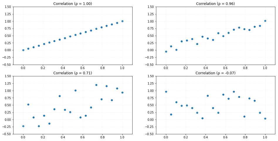
return cov/(sigma_X*sigma_Y)As an example, let's compare the correlation measure applied to random datasets. The result can vary from -1 to 1 so that values around 0 has a weak correlation and values close to -1 or 1 has a strong correlation. Negative values indicate negative correlation (decreasing slope).
Simple Linear Regression
A simple linear regression performs a treatment over two-dimensional sample points, which one represents the dependent variable $\large y$ and the other one represents the independent variable $\large x$, analytically described by:
Where $m$ describes the angular coefficient (
Where $\large \overline{y}$ and $\large \overline{x}$ are the mean values of $\large y$ and $\large x$, respectively.
Having that, we can implement the linear regression model.
class linearRegression_simple(object):
def __init__(self):
# Init class
self._m = 0
self._b = 0
def fit(self, X, y):
# Train model
X_, y_ = X.mean(), y.mean()
num = ((X - X_)*(y - y_)).sum()
den = ((X - X_)**2).sum()
self._m = num/den
self._b = y_ - self._m*X_
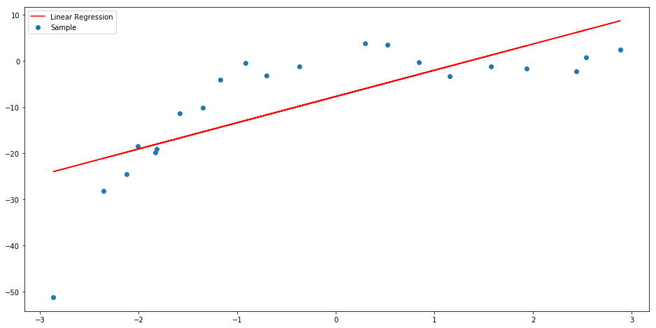
def pred(self, x):
# Predict
x = np.array(x)
return self._m*x + self._bUsing the same random datasets, we can compare the results of the linear analysis. The red line represents the linear relationship between the variables and where the new predictions would lie if we used this trained model with new independent values.
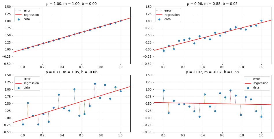
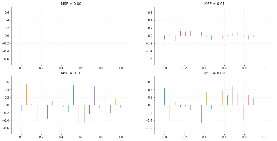
We can notice the residual lines by comparing the actual points from data and where they would be if they were predicted using our trained model. The collection of residuals provide us a very important measure called MSE (or mean squared error), which is described by:
Where $\large Y_i$ is the actual dependent value of the data point and $\large \hat{Y}_i$ is the predicted value, using the same independent variable value as an input.
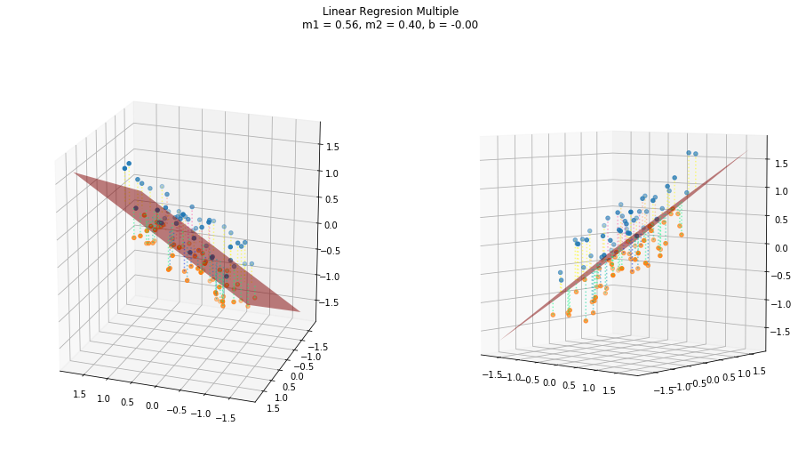
Multiple Linear Regression
A multiple linear regression performs basically the same as a simple linear regression model, but over n-dimensional sample points. This means that it has one dependent variable $\large y$, but multiple independent variables $\large x_n$, analytically described by:
Where $\large m_n$ describes the angular coefficients of each independent variable and $b$ the linear coefficient.
class linearRegression_multiple(object):
  def __init__(self):
    self._m = 0
    self._b = 0

  def fit(self, X, y):
    X_, y_ = X.mean(axis=0), y.mean(axis=0)
    num = ((X - X_)*(y - y_)).sum(axis=0)
    den = ((X - X_)**2).sum(axis = 0)
    self._m = num/den
    self._b = y_ - (self._m*X_).sum()

  def pred(self, x):
    return (self._m*x).sum(axis=1) + self._b
Using a three dimensional random datasets, we have a hyperplane that represent the linear relationship between the variables. And in the same ways as the simple regression, this plane represents where the new predictions would lie if we used this trained model with new independent values.
Gradient descent
The use of gradient descent applied to the linear regression solution is achieved by the process of minimizing the errors of the angular coefficients m and scalar coefficient b, such that:
To perform the gradient descent as a function of the error, it is necessary to calculate the gradient vector $\large \nabla$ of the function, described by:
class linearRegression_GD(object):
  def __init__(self, mo=0, bo=0, rate=0.001):
    self._m = mo     # initial value for m
    self._b = bo     # initial value for b
    self.rate = rate  # iteration's rate

  def fit_step(self, X, y):
    n = X.size
    dm = (2/n)*np.sum(-x*(y - (self._m*x + self._b)))
    db = (2/n)*np.sum(-(y - (self._m*x + self._b)))
    self._m -= dm*self.rate
    self._b -= db*self.rate

  def pred(self, x):
    x = np.array(x)
    return self._m*x + self._b
Follows a visualization of the iterative process of a gradient descent model fitting to the linear relationship.
Logistic Regression
Logistic regression is a statistical process similar to linear regression, which solves classification problems through a hypothesis about discrete values $\large y_i$, represented by:
- $\large h_\theta(x)$ is the hypothesis;
- $\large g(z)$ is the logistic function or sigmoid;
- $\large \theta_i$ is the parameters (or weights).
As similar as linear regression, logistic regression can be adjusted by gradient descent so it is necessary to calculate the sigmoid function gradient, described by:
class logisticRegression(object):
def __init__(self, rate=0.001, iters=1024):
self._rate = rate
self._iters = iters
self._theta = None
def _sigmoid(self, Z):
return 1/(1 + np.exp(-Z))
def _dsigmoid(self, Z):
return self._sigmoid(Z)*(1 - self._sigmoid(Z))
def fit(self, X, y):
self._theta = np.ones((1, X.shape[-1]))
for i in range(self._iters):
thetaTx = np.dot(X, self._theta.T)
h = self._sigmoid(thetaTx)
delta = h - y.T
grad = np.dot(X.T, delta).T
self._theta -= grad*self._rate
def pred(self, x):
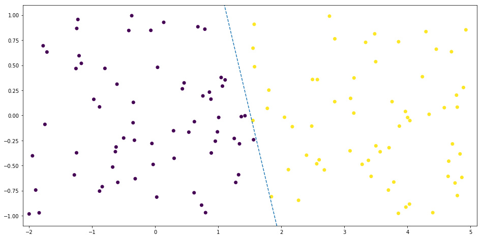
return self._sigmoid(np.dot(x, self._theta.T)) > 0.5
For the binary classification of a two-dimensional dataset, the line which describes the decision boundary is defined by:
Polynomial Regression
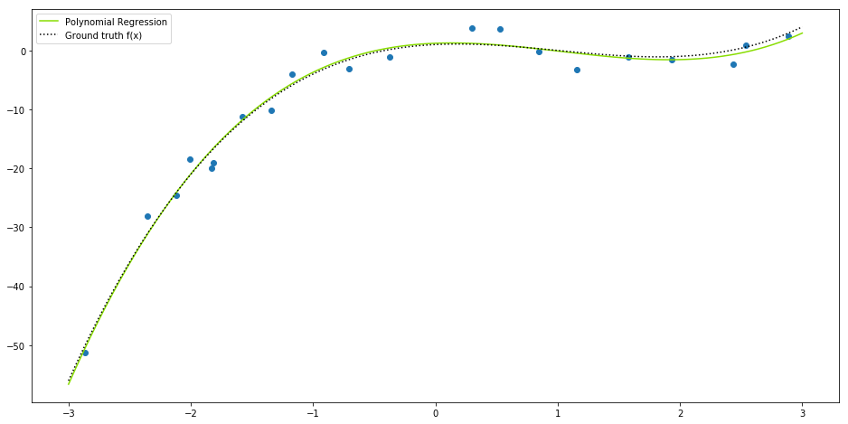
When a dataset is not linearly related or linearly separable, linear regression or logistic regression do not provide the best fit solution. For example, given the function:
If we try to apply a linear regression over the resulting data, we can notice that the linear solution does not fits very well to this.
Thus, a good option would be to use the polynomial regression, which is a non-linear prediction model, defined by:
where $\large \mathbf{X}$ (or $\large \mathbf{V}$) is the Vandermonde's matrix of the independent variable, parametrised by the maximum degree $\large m$, a response vector $\large \vec{y}$, a parameter vector $\large \vec{\mathbf{\beta}}$ and a random error vector $\large \vec{\epsilon}$. In the form of a system of linear equations, we have:
Using the Least Squares Method, the estimated coefficient vector is given by:
class polynomialRegression(object):
  def __init__(self, degree=1):
    self._degree = degree
    self._beta = None

  def fit(self, X, y):
    V = np.stack([X**i for i in range(self._degree + 1)], axis=0).T
    VTV = np.dot(V.T, V)
    VTV_i = np.linalg.inv(VTV)
    Vi = np.dot(VTV_i, V.T)
    self._beta = np.dot(Vi, y)

  def pred(self, x):
    V = np.stack([x**i for i in range(self._degree + 1)], axis=0).T
    return np.dot(V, self._beta)
Notice that our class has an attribute called degree which is the maximum degree of our function $\large f(x)$. In our example it should be $\large m=3$.